
How the fact sheets are built
A routable multimodal transportation network for Alaska — roads, local transit, intercity bus, ferry, and scheduled regional air service — is combined with U.S. Census demographics to produce one fact sheet per Alaska census place (314 communities). Every analysis runs against the same graph; numbers shown on each fact sheet trace back to the eleven-analysis pipeline below.
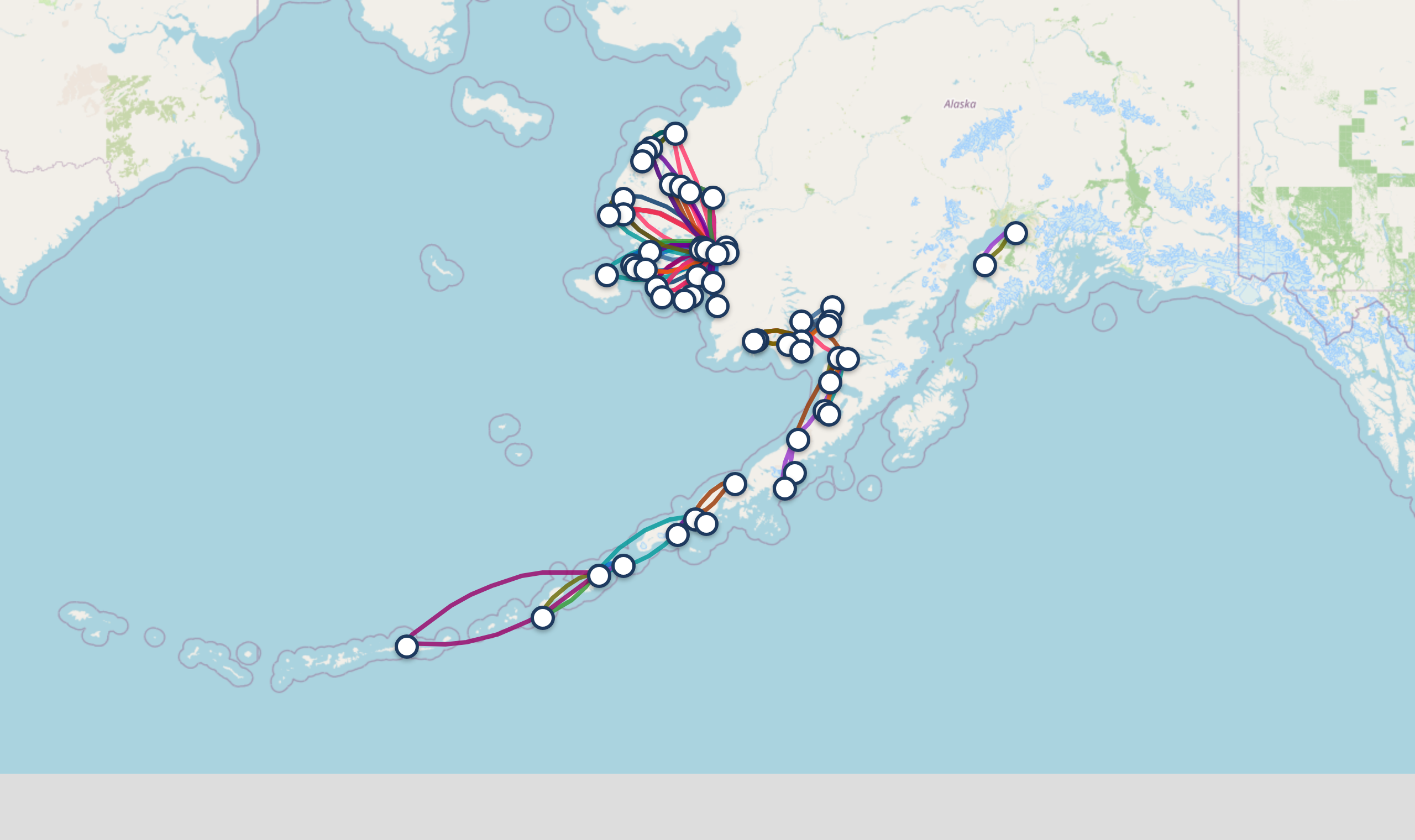
The routable multimodal network
The project is anchored on a single OpenTripPlanner (OTP) graph that fuses three OpenStreetMap road extracts (Alaska, Yukon, and a clipped portion of British Columbia covering the Alaska Highway corridor) with twenty-seven GTFS feeds — fifteen regional air carriers, ten intercity and local bus operators, and two ferry systems. Origins snap to the road-network centroid of each census place; a single multimodal graph means CAR-only and WALK + transit + air + ferry itineraries are evaluated against the same network on the same query.
Engine details
- OTP version
- 2.8.1 (jar) / 2.9.0 (Docker)
- Time zone
- America/Anchorage
- Search window
- 24 h, dynamic per community (1 h–5 d)
- Airplane board slack
- 30 min board · 20 min alight
- Walk speed
- 1.4 m/s (reluctance 4.0)
- Max journey duration
- 7 days
- Reference depart time
- 08:00, Mon 2026-01-05
- Service-frequency week
- Mon 2026-01-05 → Sun 2026-01-11
Trip cost model
Itineraries are evaluated by both travel time and estimated trip cost. Each leg's cost is computed from the per-mode rate table; the itinerary cost is the sum across legs. Costs are illustrative — actual fares vary by carrier, service tier, and discounting — but they preserve the relative magnitudes that matter for an accessibility comparison.
| Mode | Base cost / leg | Per-mile cost |
|---|---|---|
| Walk | $0 | $0 |
| Bus | $2 | $0 |
| Car | $0 | $0.70 |
| Ferry | $0 | $1.00 |
| Airplane | $115 | $1.60 |
The accessibility analyses
Eleven analyses produce the fields shown on each community fact sheet and on the statewide dashboard. Each is reproducible from the scripts in the project repo; the full consolidated dataset is published on AGOL — see the hosted feature layer for the joined CSV, GeoJSON, and shapefile.
Analysis 01Service Frequency
Counts how many scheduled flights, ferry sailings, and intercity bus trips serve each community in a representative week. Captures whether service is daily, weekly, or seasonal — the underlying signal for transit dependence and air-only access.
Method & output columns
Method
- For each Alaska census place, query OTP for transit stops within 25 km (intercity carriers) and 8 km (local transit).
- Count scheduled departures for every day of the reference week (Mon Jan 5 – Sun Jan 11, 2026) using
stoptimesForServiceDate. - Aggregate by mode: total flights / sailings / bus trips per week, plus per-day breakdowns and per-carrier counts.
- AIRPLANE-mode departures are credited if the airport is within range or reachable by car within 90 min (regional airports).
Output columns
total_flights_per_week,total_sailings_per_week,total_bus_trips_per_weeknum_air_carriers,num_ferry_services,num_bus_services+ name lists- Per-day counts:
flights_mon…flights_sun,sailings_mon…sailings_sun max_flight_gap_hours— longest scheduled gap between flights
Analysis 02Road Access
Determines whether a community is connected to Alaska's mainland road network. Communities not on the network get a straight-line distance to the nearest mainland road segment.
Method & output columns
Method
- Build a NetworkX graph from all OSM road segments in Alaska.
- Identify connected components that contain Anchorage or nodes adjacent to the Alaska–Canada border (handles Haines / Skagway).
- Buffer the mainland component by 5 km; communities falling within the buffer have road access. Off-network places report straight-line distance to the nearest mainland road.
Output columns
has_road_access— booleandist_to_mainland_road_km— for off-network places
Analysis 03Hospital Access
Travel time, cost, and best-available mode to the nearest hospital by multimodal routing. Used to bucket each community into access tiers (under 1 hour / 1–4 hours / over 4 hours / unreachable).
Method & output columns
Method
- Pre-filter to the 10 nearest hospitals by Haversine distance.
- Issue a batched OTP GraphQL request — one CAR plan and one TRANSIT (WALK + transit + air + ferry) plan to each candidate.
- Pick the option with the shortest total travel time across both modes.
- Cost = sum over legs of the per-mode rate from the cost model.
- For air-dependent communities, the transit search window is dynamically extended to cover the longest gap between scheduled flights.
Output columns
- Nearest hospital name, city
Best Travel Time (min),Best Mode,Best Trip Cost ($)- Car-route detail (time, distance, cost) and transit detail (time, cost, route summary)
- Access tier label: 🟢 < 1 h · 🟡 1–4 h · 🔴 > 4 h · ⚪ Unreachable
Analysis 04Food Access
Travel time, cost, and best mode to the nearest grocery options at three tiers — bulk food, grocery stores, and general stores — so a community's tier-by-tier proximity to fresh, packaged, and convenience food is visible at a glance.
Method & output columns
Method
- Three SNAP-retailer tiers: T1 Bulk Food (warehouse clubs) · T2 Grocery Store · T3 General Store (all other SNAP retailers).
- For each tier and each community, pre-filter to the 10 nearest stores by Haversine distance.
- Run the same batched CAR + TRANSIT OTP routing as the hospital analysis.
- Pick the shortest-time itinerary per tier; report mode and cost.
- The fact sheet renders a small Subsistence callout, tiered on
subsistence_per_capita_lbs: nothing below 150 lbs/person, otherwise “contributing” (≥ 150), “major” (≥ 300), or “primary” (≥ 500) local food source.
Output columns
- Per tier: store name, store city, store type
- Per tier: best travel time, best mode, best cost, transit route summary
Analysis 05Education Access — Local Schools
Identifies which communities have a primary or secondary school physically inside their boundary. Captures "is there a school here?" before the routing analysis answers "how far away is the nearest one?"
Method & output columns
Method
- Spatial join: each school is assigned to the census place whose polygon contains it (no buffer). Enrollment and grade span come from Alaska DEED; per-campus coordinates come from NCES EDGE Public School Locations (2023–24), because the DEED file geocodes every school to its community centroid.
- Primary (K-5) vs. secondary (6-12) classification is based on which grade-level enrollment fields are non-zero.
- Counts and total enrollment are summed per community.
Output columns
has_primary_school,num_primary_schools,primary_school_names,total_primary_enrollmenthas_secondary_school,num_secondary_schools,secondary_school_names,total_secondary_enrollmentnum_schools,school_names,total_enrollment_k12
Analysis 06Education Access — Routing
Travel time and cost to the nearest primary, secondary, and post-secondary institution by multimodal routing. Also flags whether a school of each tier is reachable within 30 minutes — a useful shorthand for communities where the school is in town vs. across a bay.
Method & output columns
Method
- Same 10-candidate Haversine pre-filter and batched OTP routing pattern as the hospital and food analyses, repeated for primary, secondary, and post-secondary institutions.
- Count institutions whose travel time is ≤ 30 min — surfaced on the fact sheet as
N school(s) within 30 min
.
Output columns
- Per tier: school name, city
- Per tier: best travel time, mode, cost, transit route summary
Primary_Within_30min,Secondary_Within_30min,Postsecondary_Within_30min
Analysis 07Transportation Infrastructure
Flags whether each community is near specific transportation features — public trails, ferry terminals, ports & harbors, USACE docks, railroad stations — using a 25 km nearest-feature threshold.
Method & output columns
Method
- Download DCCED Community Information Database (CID) layers and cache locally.
- Reproject everything to Alaska Albers Equal Area (EPSG:3338) for accurate distance.
- For each census place, find the nearest feature in each layer and flag the community as having that infrastructure if it is within 25 km.
Output columns
has_trail,nearest_trail_name,trail_distance_kmhas_ferry_terminal,ferry_terminal_name,ferry_terminal_distance_kmhas_port_harbor,port_harbor_name,port_harbor_distance_kmhas_dock,dock_name,dock_distance_kmhas_railroad_station,railroad_station_name,railroad_station_distance_km
Analysis 08Port Access (USACE Docks)
Indicates whether dock/harbor facilities are present near a community, from the U.S. Army Corps of Engineers national dock layer. Because that national layer over-counts minor and natural features and can mis-locate or mislabel small rural facilities, the fact sheet presents only presence (one vs. multiple) rather than a precise count or a specific named dock (AML review decision, 2026-06).
Method & output columns
Method
- Fetch USACE dock features filtered to
STATE='AK' AND FAC_TYPE='Dock'. - Buffer each census place polygon by 15 km in EPSG:3338.
- Count docks falling within each buffer; the fact sheet displays this as presence (one / multiple), not the raw count.
Output columns
dock_count— integerdock_availability— None / One / Multiple
Analysis 09National Waterway Network Access
Whether a community sits within 15 km of a USACE-designated navigable waterway — capturing river-and-coastal connectivity for freight and barge service.
Waterway access is based on the USACE National Waterway Network, which maps federally navigable channels used for barge and freight service. It does not include the many smaller rivers, sloughs, and coastal waters that communities rely on for boat and skiff travel. The absence of a mapped navigable waterway does not mean a community lacks water-based transportation.
Method & output columns
Method
- Fetch the National Waterway Network feature service (Alaska segments).
- Buffer each census place polygon by 15 km.
- Count intersecting waterway segments; flag communities with at least one.
Output columns
has_waterway_access— booleanwaterway_segment_count— count of NWN segments within 15 km
Analysis 10Winter Trail & Ice-Road Access
For Alaska's road-disconnected interior, winter trails and ice roads are real infrastructure. This analysis builds a graph of trail-connected communities and reports each community's nearest trail neighbours.
Method & output columns
Method
- Combine trail line layers (NWAB winter trails + Iditarod) into a single multi-line layer.
- Merge nearby same-named segments (2 km endpoint clustering, MST connectors), reducing 285 raw segments to 103 logical trails.
- Snap communities to the trail network at a 2.5 km threshold using Census Bureau interior points.
- Build a graph with intersection nodes added where trails cross; Dijkstra finds shortest network distance between trail-connected pairs.
- Layer DCRA Community Transportation Overview narratives on top — winter trail / ice road / snowmachine flags + descriptive text.
Output columns
has_winter_trail,has_ice_roadwinter_dcra_narrative(long-form description)winter_trail_access_text(summary of nearest trail-connected neighbours)
Analysis 11Travel-Shed Population Access
How many Alaskans are reachable from each community within one and four hours, using the best mode available. Captures the practical size of a community's day-trip and overnight-trip catchment.
Method & output columns
Method
- Pre-filter destinations by Haversine distance — anything beyond 1,500 km is unreachable inside 4 h on this graph.
- For each (origin, destination) pair, query OTP twice in a batched GraphQL request — one CAR plan and one TRANSIT plan, 40 destinations per request (80 plan calls).
- Pick the shorter duration per destination; depart 08:00 Mon 2026-01-05.
- Include the origin itself (0 min trivially).
- Sum ACS population for destinations under 1 h and under 4 h; count distinct communities reached.
Output columns
pop_within_1h,pop_within_4h— total Alaskans reachablecommunities_within_1h,communities_within_4h— count of communities reached
Reference frame & reproducibility
Routing queries depart at 08:00 Alaska time on Monday, January 5, 2026. Service-frequency counts span the full week Mon Jan 5 – Sun Jan 11, 2026. Air-dependent communities use a per-community search-window extension sized to that community's longest scheduled flight gap, so OTP can find the next departure even on routes that fly only twice a week.